This is part 3 in a series on machine learning. You might want to start at the beginning if you just arrived here.
In the previous post we learned about linear regression and the iterative way that a machine learning system improves its model.
As the system is trained, our aim is to minimise what is known as loss.
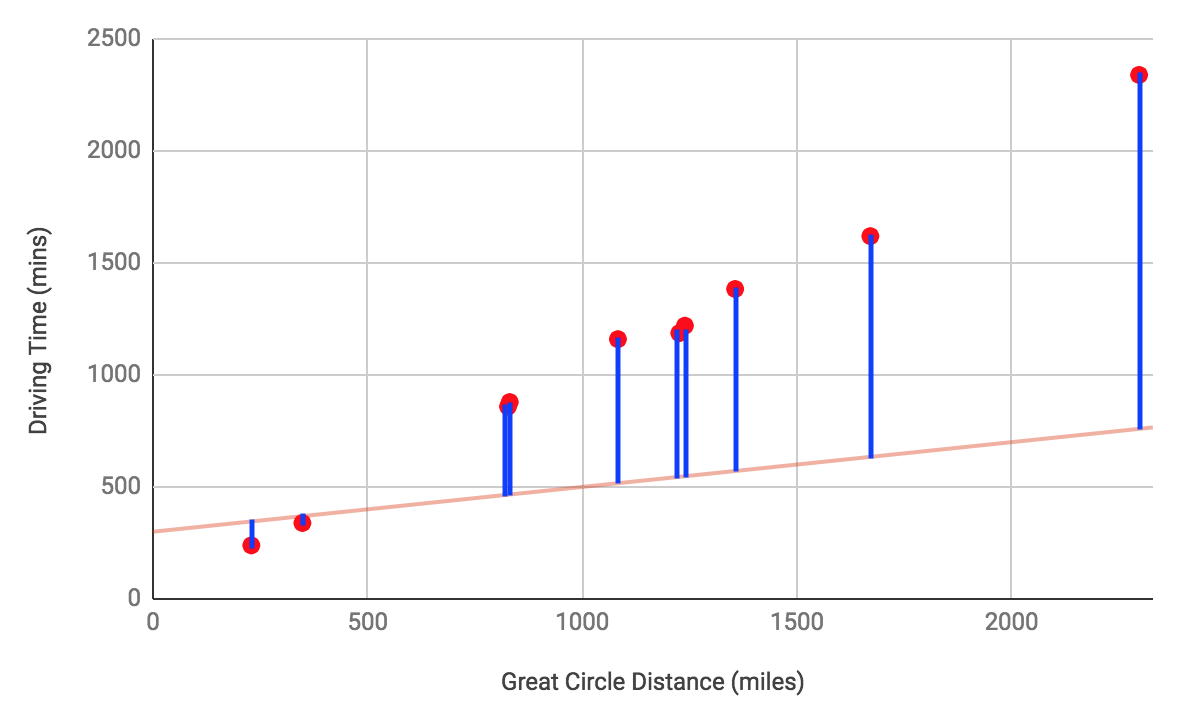
Loss is a measurement of the differences between the model’s predictions and the actual values in the training set. It’s represented as the blue lines in this graph of a model early in the training process:
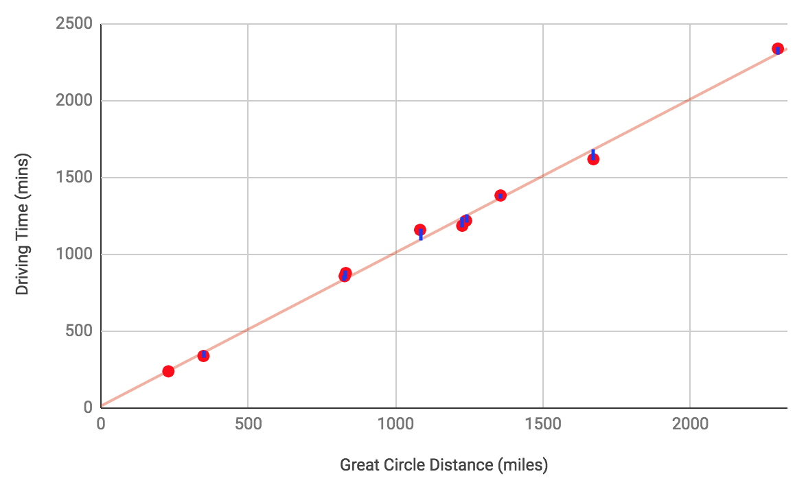
Late in the training process, when the model is a much better fit to the training data, the loss is significantly reduced:
A function known as a loss function measures loss. A common loss function is called squared loss, and it’s calculated by taking the square of the difference between the predicted value and the actual value:

To measure how the model is performing across all the training data, the Mean Squared Error can be calculated, which is simply the mean of the squared loss values:

where:
 is the Mean Squared Error
- there are
 features in the training data
  is the actual value of the
  th feature in the training data
 is the predicted value of the th feature in the training data
Once we’ve measured the Mean Square Error for a model, we adjust the weights in the model and repeat, until the model converges – which is when the Mean Squared Error stops changing or only changes by a very small amount.
Gradient Descent
Imagine you’re lost part-way up a mountain and you’re surrounded by fog. You can’t see more than a few feet in front of you. You know that if you descend the mountain you will be closer to civilisation and safety. You could walk in a random direction, but if you did then you might walk around the mountain or even start climbing it! It would probably make more sense to walk down the mountain. You might do so by looking which way the ground is sloping where you are, taking a few steps down the slope, and then reassessing which way to go.
Training a model is a similar process. We want to reduce the loss, and the only way to do so is to adjust the weights in our model. We could try guessing how to adjust the weights, but just like the climber lost on the mountain guessing which way to walk, this wouldn’t be very efficient. Instead, we can use the magic of calculus to suggest the most effective way to adjust the weights. Specifically, we use calculus to give us the gradient of the loss function. The gradient is a vector with as many dimensions as the model has weights. It’s effectively telling us how we should adjust those weights to increase the loss function in the direction of the maximum rate if increase. We want to reduce the loss, so we adjust the weights by multiplying the gradient by a small negative number – meaning that we will be adjusting the weights away from the direction in which the loss function is increasing most steeply.
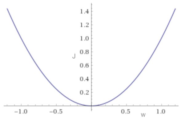
If our model had only one weight, then the loss function might look like a U shape:
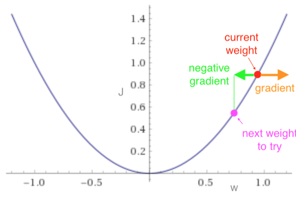
The gradient at any point gives the direction along the x-axis in which the loss function is increasing. If we adjust the weight in the opposite direction then the loss function should reduce:
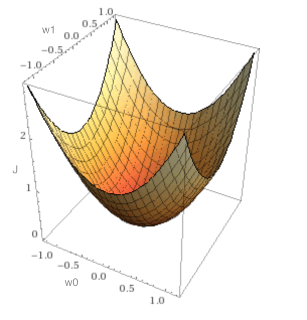
If our model had two weights, then the loss function might look like a bowl shape. The gradient at any point on the bowl points “up the hill.” We move the weights in the opposite direction, as our aim is to find the bottom of the bowl.
It turns out that the effectiveness of the training depends on the size of the adjustments we make to the weights as we’re doing gradient descent. To calculate the adjustment, we multiply the gradient by – where is called the learning rate.
If our model has two weights, the gradient is  and is 0.1 then we’ll adjust the weights as follows:

It’s important to get the learning rate right. If it’s too small then the training process will take a long time. If it’s too large then we might end up overshooting the minimal loss – like bouncing around the bowl from side to side, or even climbing out of it! We want the learning rate to be in the “goldilocks zone” – if the girl in the fairy tale was performing machine learning instead of eating porridge, she’d want the learning rate to be not too small, and not too big, but just right!
The learning rate is a hyperparameter. Hyperparameters are dials that the data scientist running the machine learning can adjust to change how the training process runs.
Next time, we’ll look at some useful ways to modify the way that gradient descent works.