This is part 2 in a series on machine learning. The first part is here.
We’re going to look at two big categories of machine learning in this series: classification and regression.
In classification the system labels the input. For example, it might label a picture as ‘cat’ or ‘dog’. There’s a discrete number of labels that the system can apply to the input.
In regression the system produces a value from a continuous range. For example, it might estimate the market value of a house in dollars based on properties such as the area of the house, the number of bedrooms, its age and so on.
Linear regression is a type of regression that models the relationship between one or more independent variables (the inputs – like the properties of a house) and a dependent variable (the output – like the estimated market value).
Let’s look at a simple example. The example will include just one independent variable and so you might be left wondering why a system would have to be trained to spot the relationship in the data. But real-world machine learning is much more complex. It often uses thousands of independent variables – far too many for any human to reason about!
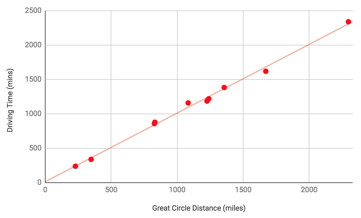
The following table shows the great circle distances and driving times from Los Angeles to a number of other cities in North America:
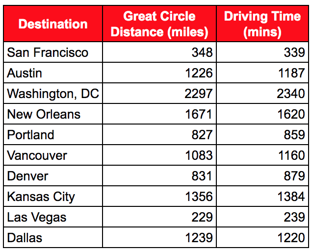
With this data, we could try and produce a model that predicts driving time based on great circle distance. The model would have one independent variable – the great circle distance – and one dependent variable – the driving time.
Before we look at how machine learning might produce a model, let’s plot the data on a graph. Humans are very good a spotting patterns in simple data, and so this can be a very powerful technique when manually investigating data. The typical convention is to plot the independent variable on the x-axis and the dependent variable on the y-axis.
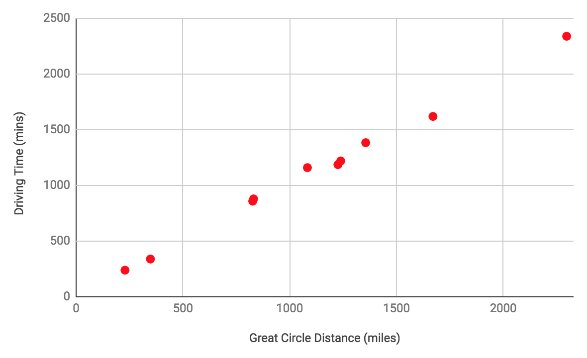
The relationship between the two variables is very easy to see when the data is plotted like this. You probably learned at school to draw a straight line through the points and express the equation for that line as

where:
 is the driving time – the dependent variable
 is the gradient of the line
 is the great circle distance – the independent variable
 is the y-intercept of the line
By convention, in machine learning we write the equation slightly differently:

where:
 is the output
 is the bias
 is the weight of the first feature
 is the first feature
This allows us to easily extend the equation when there are more features and weights.
Because a machine learning system can’t simply look at a graph to see the relationship (and because the data is usually too complex to do that anyway), it must use another approach. It uses trial-and-error by starting off with a guess and then improving that guess repeatedly until it has reached the best guess it can with the resources available to it. This is the process of training, and the guesses that the system is making are the values for the weights in the model. In this case there are just two weights to train: and .
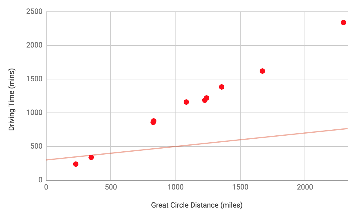
The training process will start off with poor values for and , perhaps  and
and  . The model is shown as a red line on this graph and you can see that it’s not a good fit for the data:
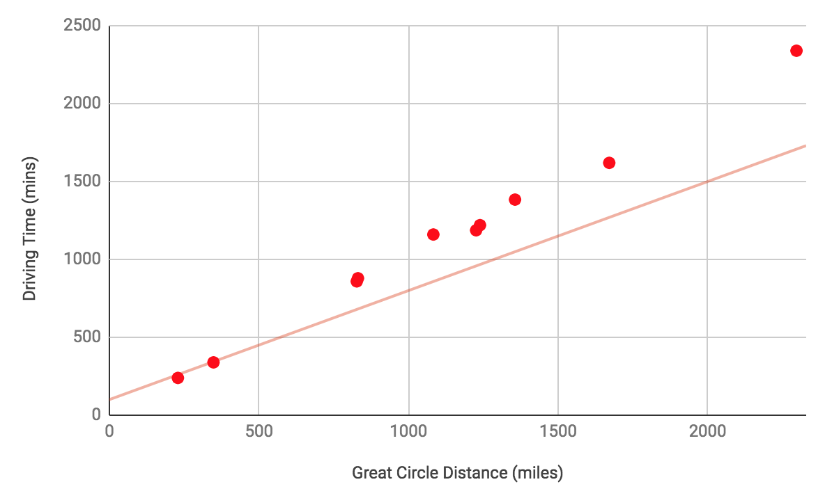
After more training, the model might look like  and
and  , which is a better fit for the data:
Eventually, after even more training, the model might become a very good fit for the data, with  and
and  :
:
To find out how the machine learning system improves the model, we’ll need to learn about loss and gradient descent – which we’ll do next time!