This is part 4 in a series on machine learning. You might want to start at the beginning if you just arrived here.
Last time around we covered gradient descent. In summary we build a model, evaluate how closely it models the training data, adjust the weights in the direction that should reduce the error in our model by the greatest amount, and repeat until the model converges.
Calculating the gradient with respect to all the elements in the training data is called “batch gradient descent.”
There are a couple of issues with batch gradient descent.
Firstly, with real world datasets it’s too slow. Our model could have thousands or even millions of weights, and the gradient is a vector with as many dimensions as there are weights in our model. In addition, the training data may have many elements, so calculating the gradient with respect to all of the data can be a very slow operation.
Secondly, our gradient may have saddle points. A saddle point is an area where the gradient is 0 or very close to 0.
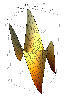
If the gradient descent passes through a saddle point then the learning may get “stuck” and we may think the model has converged even though there are other places where the loss function would be smaller.
Stochastic Gradient Descent
SGD is a modified form of gradient descent that can help with these issues. On each iteration we calculate the gradient with resepect to just one element and adjust the weights accordingly. The elements in the dataset are shuffled so they are evaluated in a random order. The gradient at some elements may be outliers and take the weights away from the global minimum. However the fluctuations in path will average out as the entire dataset is evaluated and we will usually converge on a good solution. What’s more, the fluctuations in path can help prevent the model getting stuck at a saddle point.
Mini-Batch Gradient Descent
MB-GD is a compromise between Batch Gradient Descent and SGD. With MB-GD the elements are randomly assigned to groups of  elements. On each iteration the gradient is calculated with respect to a different group. This produces a path that usually fluctuates less than SGD but is quicker to calculate than Batch Gradient Descent.
Note that Batch Gradient Descent and SGD are special cases of MB-GD where  and
and  respectively.
Momentum
Imagine a ball rolling down a hill. If you take a snapshot of the ball at any point in time then its velocity over the coming second is not simply a function of the gradient of the hill at its current location. Its current velocity also helps determine its future velocity.
Momentum in gradient descent uses a similar principle. The adjustment to weights is not just a function of the gradient at the current step but also the rate of adjustment at the previous step.
Without momentum, the update to the vector of weights  at timestep
  is as follows:

With momentum, a rate of change  is calculated that depends on the rate of change at the previous timestep:

The weight vector is then adjusted according to that rate of change:

Here  controls how much momentum the gradient descent has, with
  representing the case without any momentum.
If a saddle point is encountered with  then the gradient descent is more likely to find its way off the saddle point due to the velocity it had from earlier steps.
Nesterov Accelerated Gradient Descent
This is a variation on momentum where we evaluate the gradient at the point where the existing momentum would take us.

Until this point we’ve written  to mean the gradient at the current point in the loss function curve – more formally we would write
  . With Nesterov Accelerated Gradient Descent you can see we’re calculating it at a different point. It’s like we’re anticipating where the model parameters are going to end up, and are adjusting the rate of change in preparation for what the loss function curve will look like on the next iteration. It seems like a small change, but it makes a significant difference in real-world machine learning.
And that’s about it for today’s post. Next time we’re going to get started with some simple linear regression experiments in python!