Naive Bayes Classification

This is part 7 in a series on machine learning. You might want to start at the beginning if you just arrived here.

In the previous post we ran a linear regression on some driving distance data. We’ll return to linear regressions later, but for now let’s switch tack to classifications.

If you recall, classification is the process of applying labels to an input. As an example, let’s consider a system that has been trained with a person’s preference for various music tracks. The labels are mutually exclusive: whether the person likes the track and whether the preson dislikes the track. Each music track has been tagged according to the instruments that play in it: a singer, a guitar, a piano or drums. We’ll be able to use this system to predict whether the person will like or dislike any other track, depending on the instruments that play in it.

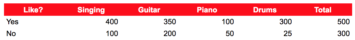
Imagine we’ve logged the person’s preference for 800 tracks so far. 500 were liked and 300 were disliked. Of the ones that were liked, 400 contained singing, 350 a guitar, 100 a piano and 300 drums. Of the ones that were disliked, 100 contained singing, 200 a guitar, 50 a piano and 25 drums.

Now let’s say there’s a track that the person hasn’t heard yet, containing singing, a guitar and drums. Do we think the person will like or dislike it?

Naive Bayes is the name of a fast and simple classifier that can give us an answer. Common uses for Naive Bayes include classification of text documents, such as classifying emails into spam or not-spam, and medical diagnosis, such as classifying observations of growths into malignant or benign.

The Bayes part of the name comes from the fact that it uses Bayes’ theorem to assign probabilities for different labels based upon the features in the input. Commonly, the label with the highest probability is the one that is selected. The Naive part of the name comes from a key assumption, that the features are independent of each other. For our music example, this means that the classifier assumes that whether a track features a singer is independent of whether it features a piano. This might be completely wrong – perhaps the 150 tracks containing a piano are all solo piano pieces and none of them features a singer. Despite this, we can still get good results with Naive Bayes, and the assumption allows the classifier to be simpler and faster, and to work with much smaller sets of training data, particular where there’s a large number of features or the values of the features vary dramatically.

Let’s look at the theory, before applying Naive Bayes to our music example.

We’ll start with the following definitions:

$K$ – the number of possible labels – in our example $K$ is 2
$C_1, C_2, C_3, ... , C_K$ – the labels – in our example these are Like and Dislike
$n$ – the number of features in the input – in our example $n$ is 4
$x_1, x_2, x_3, ... , x_n$ – the features – in our example these are Singing, Guitar, Piano and Drums

What we want to find is the probability of $C_k$ where $k = 1, 2, ... , K$ so that we can select the most likely label for the unheard music track.

The probability that a label $C_k$ should apply given the features of the track is written as:

$P(C_k | x_1, x_2, x_3, ... , x_n)$

(the notation $P(A|B)$ is used to mean the probability of A given that B has happened)

This is quite a mouthful so we’ll call it $P_k$ .

Bayes’ theorem states:

$P(A|B) = \displaystyle \frac{P(A) P(B|A)}{P(B)}$

Substituting $A=C_k$ and $B=x_1, x_2, x_3, ... , x_n$ into Bayes’ theorem gives:

$P_k = \displaystyle \frac{P(C_k) P(x_1, x_2, x_3, ... , x_n|C_k)}{P(x_1, x_2, x_3, ... , x_n)}$

We will ignore the denominator because it does not vary from one label to another, and we’re building a classifier where the actual probabilities don’t matter as long as they are proportional to each other so we can pick the most likely label. So:

$P_k \propto P(C_k) P(x_1, x_2, x_3, ... , x_n|C_k)$

We can now use the conditional probability formula, which states:

$P(A|B) = \displaystyle \frac{P(A,B)}{P(B)}$

(the notation $P(A,B)$ is used to mean the probability of both A and B happening – note that we don’t know whether or not B has happened, whereas in $P(A|B)$ we know that B definitely has already happened)

Substituting $A=C_k$ and $B=x_1, x_2, x_3, ... , x_n$ into the conditional probability formula gives:

$P_k\propto P(x_1, x_2, x_3, ... , x_n, C_k)$

Reusing the conditional probability formula with $A=x_2, x_3, ... , x_n, C_k$ and $B=x_1$ we get:

$P_k\propto P(x_1 | x_2, x_3, ... , x_n, C_k) P(x_2, x_3, ... , x_n, C_k)$

and repeatedly applying the same technique we end up with:

$P_k\propto P(x_1 | x_2, x_3, ... , x_n, C_k) P(x_2 | x_3, x_4, ... , x_n, C_k) ... P(x_{n-1} | x_n, C_k) P(x_n | C_k) P(C_k)$

This is where the naive assumption kicks in. If we assume that none of $x_2, x_3, ... , x_n$ impact the likelihood of $x_1$ then we can say:

$P(x_1 | x_2, x_3, ... , x_n, C_k) = P(x_1 | C_k)$

Applying this to each term we get:

$\begin{align*} P_k &\propto P(x_1 | C_k) P(x_2 | C_k) ... P(x_{n-1} | C_k) P(x_n | C_k) P(C_k) \\ &\propto P(C_k) \prod\limits_{i=1}^{n}{P(x_i | C_k)} \end{align*}$

Commonly in a classifier the maximum a posteriori approach is used, which is a fancy way of saying that we’ll pick the label that has the largest probability. In mathematical terms:

$y' = \underset{k \in \{ 1, ..., K\}}{\text{argmax}} P(C_k) \prod\limits_{i=1}^{n}{P(x_i | C_k)}$

That was a lot of theory, so let’s apply it to our unheard music track.

It contains singing, a guitar and drums. So we need to calculate:

$P(Like) P(Singing | Like) P(Guitar | Like) P(Drums | Like)$ and

$P(Dislike) P(Singing | Dislike) P(Guitar | Dislike) P(Drums | Dislike)$ and pick the label that has the larger value.

$\begin{align*} P_{Like} &= \frac{500}{800} \frac{400}{500} \frac{350}{500} \frac{300}{500} = 0.21\\ \\ P_{Dislike} &= \frac{300}{800} \frac{100}{300} \frac{200}{300} \frac{25}{500} = 0.00694...\\ \end{align*}$

Clearly Like has the larger value, so this model predicts that the person will like the music track when they hear it.

Hope you made it through the theory and the worked example! Next time we’ll run some real Naive Bayes using python.

Mark Fryer

Naive Bayes Classification

Leave a Reply Cancel reply