This is part 9 in a series on machine learning. You might want to start at the beginning if you just arrived here.

Last time we built a model to predict whether a tumour was benign or malignant.

There is a way we could have built a model that was trivial to create and that successfully identified 100% of the malignant tumours. Sound too good to be true? Well, unsurprisingly, it is. For the model being considered here is one that simply returns “malignant” for all tumours. And the cost would be incorrectly predicting malignancy for all of the tumours that actually turned out to be benign.

So when we’re looking at how suitable a model is for things such as binary classification, we need to look at how many of the selected items are relevant (how many of the tumours predicted to be malignant are actually malignant) as well as how many of the relevant items were selected (how many of the malignant tumours were predicted to be malignant).

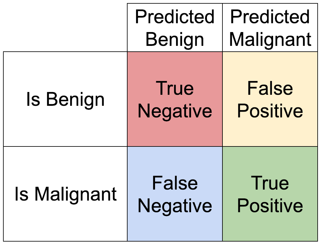
We can summarise this in a simple truth table. The rows represent the two possible states for each tumour, often called the target variable. And the columns represent the two possible predictions for each tumour.

We can define two ratios that together can be used as an indication of how the model is performing.

The first ratio is Recall. Recall is the proportion of relevant items that were selected. The number of true positives divided by the number of malignant tumours.

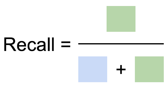
Recall is also known as Sensitivity.

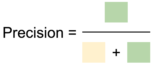
The second ration is Precision. Precision is the proportion of selected items that are relevant. The number of true positives divided by the number of tumours predicted to be malignant.

The trivial model that returns “malignant” for all tumours has perfect recall. But it has terrible precision.

At the other end of the spectrum, a model that only predicts a tumour is malignant when the evidence is overwhelming might have a good precision but a poor recall.

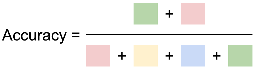
Neither of these ratios considers the number of True Negative predictions in our truth table, and so they can be vulnerable to manipulation. An alternative measure, which considers all the counts in our truth table is known as the Rand Index or Rand Accuracy or simply Accuracy. It calculates the proportion of predictions that were correct.

The final ratio that we’ll cover here is Specificity. Specificity is the proportion of actual negatives that are correctly identified. The number of true negatives divided by the number of benign tumours.

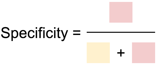
Sensitivity (another name for Recall) and Specificity are often quoted in medical tests. A good medical test will have a high sensitivity (most people with the condition are correctly identified) and a high specificity (most people without the condition are correctly identified as such). For a medical test, it can be very important to avoid false positives due to the potential stress that a false positive diagnosis can cause, and so a high specificity is demanded. In other situations, a false positive might be less costly and so a comparatively low specificity might be accepted as a side-effect of tuning the test to drive a high sensitivity.

The trade-off between sensitivity and specificity can be plotted on an ROC curve (Receiver Operating Characteristics). This curve plots True Positive Rate (TPR), also known as Recall / Sensitivity against False Positive Rate (FPR) which is 1 – Specificity. If you have a model whose decision threshold can be varied then each value of the decision threshold produces a pair of TPR and FRP values, which can then be plotted on the ROC curve.

For example, if you are screening people at a security checkpoint, varying how strictly you screen the people is a case of varying the decision threshold – the decision being whether to prevent them from passing through the checkpoint. As the decision threshold varies, the numbers of True Negatives, False Negatives, False Positives and True Positives change:

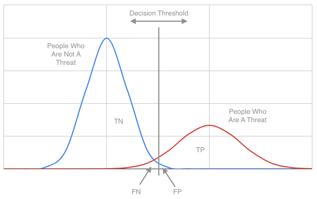
If you only stop people when they are very clearly carrying a weapon then you will have high specificity (few false positives: most people you stop will be a threat) and low sensitivity (lots of false negatives: people who hide weapons well get through the checkpoint). If you stop people when there’s the slightest chance that they are a threat then you will have low specificity (many false positives: lots of innocent people will be stopped) and high sensitivity (few false negatives: few people with a weapon will get through).

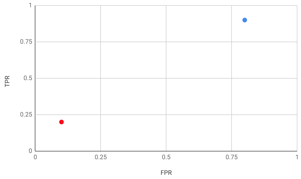
These two cases are plotted on the above ROC curve. The red dot represents the first case, where the security threat had to be very obvious before the person would be stopped. And the blue dot represents the second case, where the slightest suspicion caused the person to be stopped.

Nirvana on an ROC curve is the top left corner, with high sensitivity and high specificity. Interestingly, the bottom right corner is paradoxically good too, because the predictions can be reversed in order to put the model into the top left corner. Where you don’t want your model to be is close to the line y = x, because there your model is doing no better than random guesses.

So we can have a good model where the threats and not-threats are quite clearly distinguished when the decision threshold is adjusted:

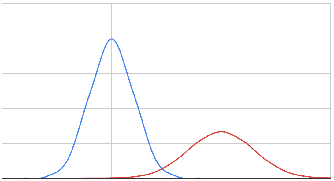
And we can have a bad model where there is a lot of overlap between the two sets of people:

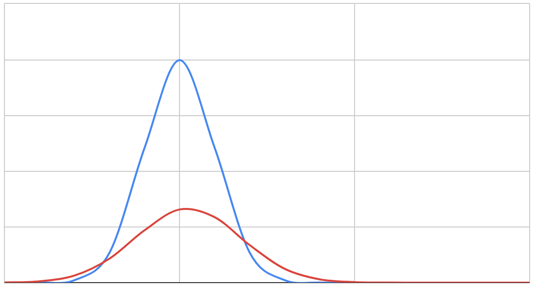
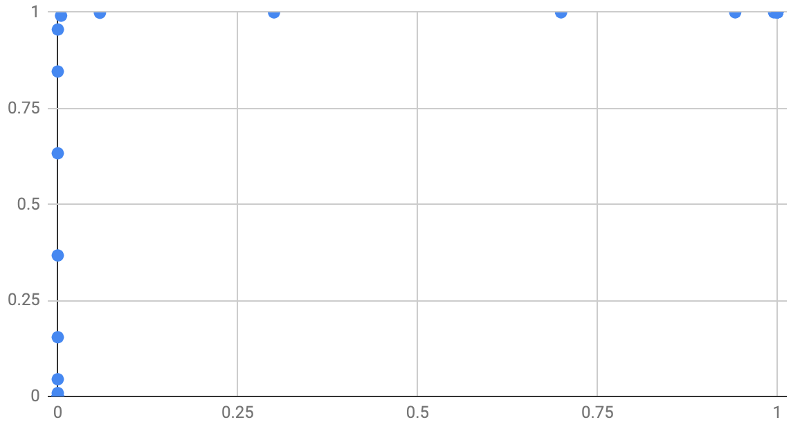
And these have two very different ROC curves. Here’s the good model’s ROC:

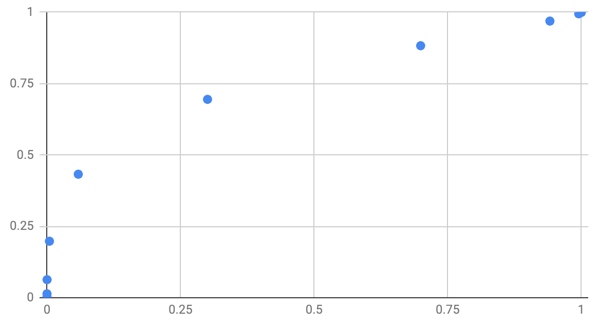
And here’s the bad model’s ROC:

This leads to the final metric I’m going to introduce today, which is the Area Under the ROC or AUROC – often simply called Area Under the Curve or AUC. It’s taken from the area below the curve plotted on the ROC curve. The higher the AUC, the more useful the model is at classifying the input data. A perfect classifier has an AUC of 1. A classifier that guesses randomly has an AUC of 0.5. A classifier that’s wrong every time has an AUC of 0.

When choosing a classifier you want to have an AUC as far as possible from 0.5. If it’s close to 1 then great. If it’s close to 0 then you can invert the decision your model is making and you’ll get a new model with an AUC close to 1.